Difference between revisions of "Example: Absolute Solvation Free Energy"
| Line 3: | Line 3: | ||
This page will guide you through the process of designing a simple free energy simulation. In particular, this example will set up an OPLS-AA forcefield simulation of ethanol in a box of TIP3P water. The purpose of this page is not to take you through step-by-step the process of simulation, but instead guide you through the logical decisions that can be applied to any simulation package of your choosing. | This page will guide you through the process of designing a simple free energy simulation. In particular, this example will set up an OPLS-AA forcefield simulation of ethanol in a box of TIP3P water. The purpose of this page is not to take you through step-by-step the process of simulation, but instead guide you through the logical decisions that can be applied to any simulation package of your choosing. | ||
| − | See also [[GROMACS 4.6 example: Direct ethanol solvation free energy|instructions on how to run this calculation with | + | See also [[GROMACS 4.6 example: Direct ethanol solvation free energy|instructions on how to run this calculation with GROMACS 4.6]] using standard free energy calculations, or using [[GROMACS 4.6 example: Ethanol solvation with expanded ensemble|using expanded ensemble simulations]]. |
Let's start with the visuals of the system, we want to simulate a box of TIP3P water where an ethanol molecule is appeared inside the box. | Let's start with the visuals of the system, we want to simulate a box of TIP3P water where an ethanol molecule is appeared inside the box. | ||
Revision as of 21:29, 15 April 2013
| Free Energy Fundamentals |
|---|
 |
|
Methods of Free Energy Simulations
|
| Free Energy How-to's |
|---|
 |
This page will guide you through the process of designing a simple free energy simulation. In particular, this example will set up an OPLS-AA forcefield simulation of ethanol in a box of TIP3P water. The purpose of this page is not to take you through step-by-step the process of simulation, but instead guide you through the logical decisions that can be applied to any simulation package of your choosing.
See also instructions on how to run this calculation with GROMACS 4.6 using standard free energy calculations, or using using expanded ensemble simulations.
Let's start with the visuals of the system, we want to simulate a box of TIP3P water where an ethanol molecule is appeared inside the box.
What is the Thermodynamic Cycle?
The first thing we must do is define which path we will carry out our simulation under. There are two main paths we could take:
Direct Caclulation
Intermolecular interactions are eliminated between the water and ethanol.
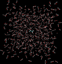
- End State A) Fully interacting system where the ethanol is interacting with every water.
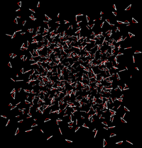
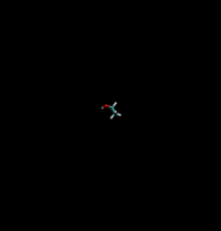
- End State B) Ethanol interacts with itself and is free to move around the box as if the water was not there, and water interacts with itself and acts as if the ethanol is not there.
- Effectively, the interactions would look like the following between the two states
|
|
| ||
| State A | State B | |||
Indirect Calculation
Disable ALL the ethanol interactions, then do it again in vacuum so you can add the forces back into the calculation. Recall that intramolecular interactions must remain on to be accurate. For this, we need four total states,
- End State I-A) Fully interacting system where the ethanol is interacting with the water.
- End State I-B) Ethanol is annihilated leaving only water to interact with itself.
- End State II-A) Vacuum system where ethanol is allowed to interact with itself.
- End State II-B) Ethanol is annihilated in vacuum, leaving no interactions.
- Visually:

|

| |
| State I-A | State I-B | |

|

| |
| State II-A | State II-B | |
What are the End States?
The end states are shown above and depend on the thermodynamic cycle chosen. One may ask "why would you ever choose the Indirect calculation?" since it requires seemingly more steps. The answer will usually depend on the software you are using. Free energy calculations are not always implemented in code and the software may not be able to define a system with only selective interactions (i.e. you get either all atoms interacting together or you get none).
Even if you must do the annihilation runs, vacuum simulations with one molecule are often very quick and efficient, so there is a negligible increase in total computation time.
What are the Intermediate States?
Defining the intermediate states are one of the most challenging parts of any free energy calculation, and each method shown above will have different (although very similar) states.
For the Direct Calculation, a robust way would be to:
- Linearly turn off intermolecular charge interactions of the ethanol with the solvent.
- Scale the van der Waals interactions from ethanol to the solvent by a soft core potential.
For the Indirect Calculation, a slightly different but equally robust scheme would be:
- Linearly scale the charges on ethanol to zero (Note: this fully disables the charge as opposed to remove interacting with only one type of molecule).
- Turn off the Lennard-Jones interactions with a soft core transformation.
- Repeat this process in vacuum.
Since the bonded interactions are not changing, there is nothing special that needs done for this in either case.
The number of intermediate states will depend on length of simulation, free energy method used, and exact form of soft core potential. Take for example either BAR or MBAR; 3-5 charge terms and then 5-8 Lennard-Jones terms for a small molecule like benzene or toluene would be sufficient to give errors in the 0.1-0.05 kcal/mol range with 5 ns simulation time at each [math]\displaystyle{ \lambda }[/math] state. This level of precision was attained in previous large scale studies with the caveat that [math]\displaystyle{ \lambda }[/math] spacing was chosen to minimize variance.[1]
Under equal [math]\displaystyle{ \lambda }[/math] spacing, you will likely need more states, something to the order of 10 for the charge and 20+ for the Lennard-Jones. This emphasizes how important choosing [math]\displaystyle{ \lambda }[/math] spacing to the efficiency of your simulations. However, there is still the tradeoff in available resources as adding more states requires; it should be noted that TI would likely require more intermediates than BAR or MBAR to achieve the same level of uncertainty.
What Simulations to Run?
Each and every intermediate and end state must be equilibrated first. Typically, one could start with the fully interacting state at all intermediates, and run for perhaps 1 ns, to allow the system to equilibrate. Alternately, one could prepare each configuration at each intermediate state to run sequentially, then equilibrate each of those for the 1 ns.
The simulation box should be large enough to prevent any molecule from interacting with itself, meaning the width of the box should be twice the cutoff length plus the longest width of the molecule.
Required simulation time will depend on the accuracy of the simulation. For this example and a target uncertainty of < 0.1 kcal/mol, 5 ns of simulation at each [math]\displaystyle{ \lambda }[/math] value will likely be sufficient if the time scales for torsional rotation are not too large.
What Analysis do we Perform?
For this example, lets assume we are using BAR and the code does not automatically print out energy differences. In this case, the potential energy differences must be generated by single point simulations. This can be done by saving configurations every N steps, where 'N will depend on the correlation times of the potential energy. Typically, for a small rigid molecule, it will be around 1-10 ps, though longer if there are slow degrees of internal freedom.
Once you have the configurations, you will then run point energy calculations. These calculations should be identical to the ones performed to generate the runs, except that each configuration will also be evaluated at the [math]\displaystyle{ \lambda }[/math] value of the neighboring intermediate. For each interval, we will have two energy differences:
- The difference from state i to i+1 sampled from state i
- The difference from state i+1 to i sampled from state i+1
The BAR calculation is performed for each interval to get the free energy difference between each adjacent state. We could then run bootstrap sampling to the data set of evaluated energies to get an error estimate that way. If the energy difference is printed out, we can skip everything up to this point and just run the bootstrap sampling and BAR calculation, simplifying and speeding the analysis process.
Catches, Traps, and Anything to Watch out for
At the end state, ethanol will be isolated from the rest of the system, so you cannot exchange its kinetic energy with the rest of the system. With particular choices of thermostat, kinetic energy can get transferred between the isolated subsystems in a way that violates equipartition. The degrees of freedom of the water and the ethanol should either be thermostated independently, or more robustly with a Langevin or other stochastic thermostat like the Andersen thermostat. [2]
Long range interactions must also be considered, notably the dispersion effects. One may think that these are not important since they drop off as [math]\displaystyle{ r^{-6} }[/math], however, they can play a significant role, adding up to 0.5-1 kcal/mol for small molecule solvation free energies. If not supported in the code, an analytical correction must be made to integrate the attractive part of the van der Waals term out to infinity. If the system is nonisotropic, then even the analytical correction may be incorrect; however, there are still solutions for this. [3]
References
- ↑ Pham, T. T., and Shirts, M. R. (2011) Identifying Low Variance Pathways for Free Energy Calculations of Molecular Transformations in Solution Phase. J. Chem. Phys. 135, 034114 - Find at Cite-U-Like
- ↑ Shirts, M. R., Mobley, D. L., and Chodera, J. D. (2007) Alchemical Free Energy Calculations: Ready for Prime Time? Annu. Rep. Comput. Chem. 3, 41–59. - Find at Cite-U-Like
- ↑ Huang, N., and Jacobson, M. P. (2007) Physics-based methods for studying protein-ligand interactions. Curr. Opin. Drug Di. De. 10, 325–31. - Find at Cite-U-Like