Example: Relative Binding Affinity

Free Energy Fundamentals
Theory Definitions Exponential Averaging / Zwanzig Thermodynamic Integration Bennett Acceptance Ratio WHAM MBAR
Methods of Free Energy Simulations Thermodynamic Cycle Intermediate States (Constructing) Soft Core Potentials Running Simulations Extracting Simulation Information Analysis / Bootstrap Sampling
Improving Sampling and Accelerating Simulations Umbrella Sampling Hamiltonian Replica Exchange [math]\displaystyle{ \lambda }[/math]-dynamics / Expanded Ensemble

Free Energy How-to's
Example Calculations Absolute Solvation Free Energy Relative Binding Affinity Absolute Binding Affinity
Tutorials Ethanol Solvation - GROMACS Expanded Ensemble - GROMACS Absolute Binding Free Energy - GROMACS

This example will be a bit more complex than the solvation example since we are now transforming one molecule to another within an environment. Again, the purpose of this page is not to take you through step-by-step the process of simulation, but instead guide you through the logical decisions that can be applied to any simulation package of your choosing. We will work through the same questions that were asked on the previous example as these should be asked for any free energy simulation.

For this particular example, we will look at the difference in the relative binding free energies of toluene and phenol in the apolar cavity of T4 Lysozyme.

Toluene in the pocket...

... becomes phenol in the pocket.

What is the Thermodynamic Cycle?

Example of using a thermodynamic path to find which molecule has a stronger binding affinity. We could either remove both molecules from the pocket which is time prohibitive, or we could simply transform one molecule to another both in and out of pocket to find the difference that way.

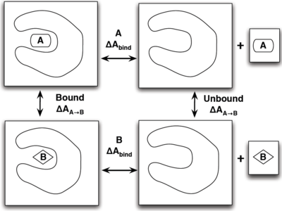
If you have already read through the thermodynamic cycle page, then you will have already seen this picture on the left. For our simulation, we can define the thermodynamic cycle either by directly converting toluene to phenol (which would be very costly due to the large number of changing interactions and box size), or we can recognize that free energy is a state function and we can use this relation to solve for it as well:

[math]\displaystyle{ \Delta \Delta A_{\mathrm{bind}} = \Delta A_{\mathrm{bind}}^B - \Delta A_{\mathrm{bind}}^A = \Delta A_{A\rightarrow B}^{\mathrm{bound}} - \Delta A_{A\rightarrow B}^{\mathrm{unbound}} }[/math]

which does not require an excessively large box and can be done relatively simply by choosing the correct intermediate states to transform the ligands.

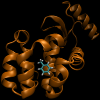
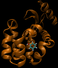
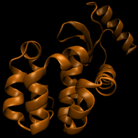
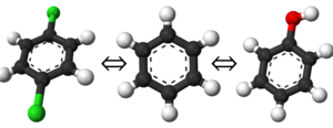
To provide the visuals for this particular system, please see the rendered images below; note that the solvent can be either implicit or explicit and the cycle will still be valid.

Molecule Visualization

To show this with the actual molecules present, the rendered image below shows the thermodynamic cycle as well

	A [math]\displaystyle{ \Delta A_{\mathrm{bind}} }[/math]
Bound [math]\displaystyle{ \displaystyle \Delta A_{A\rightarrow B} }[/math]		Unound [math]\displaystyle{ \displaystyle \Delta A_{A\rightarrow B} }[/math]
	B [math]\displaystyle{ \Delta A_{\mathrm{bind}} }[/math]

What are the End States?

There are two real end states we need here. Since the T4 lysozyme and solvent are not changing in either case, they will be present in both end states.

• State A) T4 lysozyme in solvent with an intermediate molecule that looks like toluene in the pocket.
• State B) T4 lysozyme in solvent with an intermediate molecule that looks like phenol in the pocket.

Dual topology approach. Even though the intermolecular forces will be for the real atoms, there are still dummy intramolecular forces. Please see the full page on topologies for a more in depth description.

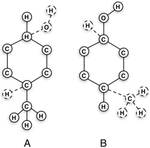
What does it mean to have an "intermediate state look like" a molecule as an end state? This intermediate state could well be just toluene or phenol, however, there will still be the dummy atoms on it based on the topology choice. Recall from the figure on the right that, even though the interacting molecule will be a physical molecule, there are still the dummy interactions that must be built in and considered.

For this example, a dual state topology is shown on the right, but it is by no means the only set of end states one could chose; an ortho- or meta- arrangement could just as easily be selected with the dual topology scheme. There is also not a limitation on just dual topologies as single topologies will also work in any of the arrangements.

Although beyond the scope of this example, it is also worth mentioning there is also research ongoing in predicting how a real molecule will behave and the end point will not have the full interactions of a real molecule, but some unphysical intermediate. The free energies of the real molecule are extrapolated from these results. This is particularly helpful for doing more than one transformation as you would not need a unique set of intermediate states for each pair of real molecule end points.

What are the Intermediate States?

For this example, we will assume that the phenol is the initial state, although we could have just as easily assumed it was the toluene. Observe that the OH moiety must disappear and the methyl must appear to make the transformation complete. A good first approach sample set of intermediates can be constructed that follow this process:

1. Turn the charge on the OH and the para- hydrogen to zero. Recall it is important to make sure the overall system is at the same total charge at each intermediate.
2. Next, you will want to turn the Lennard-Jones [math]\displaystyle{ \epsilon }[/math] on the hydroxyl and para- hydrogen turned to zero.
   • You can simultaneously turn off angle, torsional, and bonded terms linearly.
3. Now turn on the methyl's Lennard-Jones [math]\displaystyle{ \epsilon }[/math] and its corresponding para- hydrogen.
   • The corresponding angle, torsional, and bonded terms will also need turned on.
4. Lastly, turn on the charges of the methyl and corresponding para- hydrogen.

Independent of which pathway you select, you will still need a sufficient number of intermediates. By choosing BAR or MBAR as our method, we may need 2-4 intermediates for the charge and 4-6 for the Lennard-Jones changes. This is less than the ethanol solvation because there are fewer atoms changing, corresponding to better phase space overlap. TI would take roughly 2-3 times the number of intermediates. You could run both Lennard-Jones transformations at once, but you would have to first disable improper torsions first otherwise the atoms will collide with each other.

What Simulations to Run?

As with all free energy methods, start by equilibrating all intermediate states. Unlike in the solvation example though, the starting configuration is more complex since we are in a binding site as opposed to a homogeneous fluid.

The ideal starting point would be a crystal structure configuration, or a homologous ligand to which the target ligand can be approximated as without distorting either protein or ligand. When the binding site is not know, accurate free energies are not easy to obtain, if at all, and docking is not suitable for picking a single "best" binding site. That said, if the binding site is known but no crystal structure is available, then docking can be used to generate a set of potential starting configurations, You will need several nanoseconds (tens of ns ideally) to see if the starting positions interconvert. If they do not, you may have to run multiple simulations for each binding site.

After starting configurations are selected, the best option would be to start from a fully interacting state and run short simulations at each [math]\displaystyle{ \lambda }[/math] values to allow partial equilibration, then run long equilibrations at each [math]\displaystyle{ \lambda }[/math] state at constant pressure to find the equilibrium densities. For the example here, you will need 2-4 ns of equilibration because correlation times are guaranteed to be longer than the small molecule solvation test. Even if one has a crystal structure, you should test multiple starting configurations (from multiple crystal structures if possible) to see if the ligands all sample the same conformational states. This is done because different starting configurations may have very different confrontational space they sample and so you will want multiple runs to access the largest space.

Box size should again be large enough for the protein and ligand to not interact with their respective selves, which means the box's width should be twice the cutoff plus the longest width of the collective protein/ligand width. Given the size of this example, around 50 ns of simulation may be required to get consistent results (solvent representation will also affect this). At the time of writing (Oct 2012), even with relatively rigid proteins, getting results that have uncertainties less than 0.5 kcal/mol is very challenging.

What Analysis do we Perform?

For a more diverse example, we will assume we want to analyze this system by TI instead of BAR or MBAR. For this, we can usually assume that {{#tag:math|{{dudl} }} is calculated and printed at each step. If it were not calculated and we were using soft core transformations, TI would be impossible to calculate in post-processing. Because we already have the derivatives, all we have to do is average them for a given state, then perform numeric integration and error estimations by the methods discussed previously.

Relative binding free energy is then the difference between the two transformations.

Catches, Traps, and Anything to Watch out for

Visualize what your system is doing by either observing trajectories or tracking some position properties like RMSD to ensure odd things are not happening. If for instance you are trying to bind p-xylene to this pocket, you would expect the Val111 side chain to change orientation.

More generally though, very little was said about the protein for our example. One can think of the protein as just another environment that the change is occurring within. One difference that occasionally has some relevance is the location of the binding state. If the ligand is a tight binder, it will always remain very localized around the binding site, making binding site irrelevant. As for a weak binding ligand ([math]\displaystyle{ K_d }[/math] 100 µM), comparatively more time is spend outside the binding site, making the identification of a "bound" configuration very hard to define. Scientists who run simulations and those that run experiments both suffer from this difficult definition though, so you will not be alone in this regard. For weak binders, careful comparison of exactly the physical phenomena leading to signalling binding must be exported and getting quantitative results will be difficult (e.g. the Val111 and p-xylene example). For most problems of interest, determining the precise binding affinities of weak binders is not important, but the ability to distinguish between a tight and weak binder will be.

Lastly, starting simulations from the different configurations will provide information about convergence if they all converge to the same point.

References

- ↑ 1.0 1.1 Roux, B., and Faraldo-Gómez, J. D. (2007) Characterization of conformational equilibria through Hamiltonian and temperature replica-exchange simulations: Assessing entropic and environmental effects. J. Comput. Chem. 28, 1634–1647. - Find at Cite-U-Like
- ↑ 2.0 2.1 Andersen, H. C. (1980) Molecular dynamics simulations at constant pressure and/or temperature. J. Chem. Phys. 72, 2384–2393. - Find at Cite-U-Like
- ↑ Jiang, W., and Roux, B. (2010) Free Energy Perturbation Hamiltonian Replica-Exchange Molecular Dynamics (FEP/H-REMD) for Absolute Ligand Binding Free Energy Calculations. J. Chem. Theory Comput. 6 (9), 2559–2565. - Find at Cite-U-Like